Algorithmic Complexity Made Simple
G. Wade Johnson
Campbell Johnson
What is Algorithmic Complexity?
A way of reasoning about algorithm performance.
When trying to find bottlenecks in code, profiling is the way to go. Sometimes, it's not obvious why code is slow when profiling a small example. You also can't profile code that has not been written. How do you compare algorithms before you have an implementation?
The study of algorithmic complexity provides the tools needed to reason about algorithms when measurement is not enough or is not possible.
Premature optimization
Premature optimization is the root of all evil.
Sometimes also referred to as a violation of YAGNI. The general idea is that you should not waste time optimizing code if you don't know whether it matters.
Premature pessimization
Premature pessimization is the root of some evil.
Just because you shouldn't optimize prematurely, does not mean that you should write obviously bad code either.
Algorithms not micro-optimizations
Micro-optimizations often give 2-10% improvements.
Algorithm changes can give a factor of 2-10 improvement.
Although a series of micro-optimizations can actually add up to more, it's usually at a large cost in redability. Algorithmic changes can be less under some circumstances, but once in a while it can be orders of magnitude better performance. Surprisingly an algorithm with much better performance is often not any less readable.
Big O notation
Describes the worst-case behavior of an algorithm.
Highest order term in a mathematical description of the algorithm.
There are other similar ways of talking about algorithms, but Big-O is the most common. If you were to write an equation describing the performance of an algorithm in terms of the size of the input, you will find that the highest order term dominates as the input size becomes large.
Orders of Algorithms

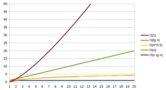
- Constant:
O(1) - Sub-linear:
O(lg n) - Linear:
O(n) - Supralinear:
O(n lg n)
Constant means that the algorithm is independent of input size (say indexing into an array). Algorithms that repeated divide their input in half generate a logarithmic order. Examples include binary search, and tree search algorithms. A linear algorithm is one that performs a constant amount of work for each item in the input.
The most familiar O(n log n) algorithms are sort
algorithms like quicksort, heapsort, or merge sort.
Orders of Algorithms, supralinear

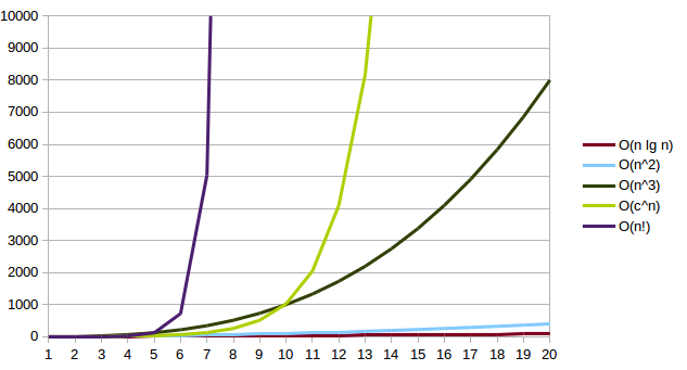
O(n2)O(nc)where c > 1O(cn)O(n!)
All of the O(nc) algorithms are pretty easy to
recognize. Look for nested loops over the input.
The O(cn) are most often found in public
key cryptography. Any time you need to work on permutations of a data
set, you get into the realm of O(n!). These more complex
algorithms are things that you really want to avoid for large data
sets.
The Math
- Count/measure the cycles/instructions executed for an implementation.
- Work out the parts of the measurements that are related to input size.
- Develop an equation describing the work done.
- Analyze equation to recognize the important features.
Who cares? In reality, no one actually does this outside of people working on microcode.
The Reality
- Apply rules of thumb to recognize important features of an algorithm.
- Pick most prominent term.
- Change or accept algorithm.
In reality, you look to see if you are heading in the right direction or are going to fall into a big hole. Based on that, you get back to delivering value.
Test 1
for my $i (@ARGV)
{
    for my $j (@ARGV)
    {
        ...;
    }
}
This is the classic case of an O(n2) algorithm.
Test 2
for my $i (@ARGV)
{
    $x += grep { ... } @ARGV;
}
Slightly less obvious, but still O(n2).
Test 3
my @out = map { ... }
          grep { ... }
          @in;
Don't let the double loop fool you, this is a linear algorithm (O(n)). We do two loops, one after the other. It's only quadratic if it were one inside the other.
Several people wondered if the number of items returned by the grep.
The first thing to remember is that big-O value is related to the worst-case. The
second thing is that this algorithm is linear not quadratic, so the order does not
actually depend on the number of items returned by grep.
Test 4
sub foo
{
    return @_[0] if @_ < 2;
    foo( @_[0 .. (@_/2)] );
}
This is an O(lg n) algorithm. Each time foo is called, it has half the input that it had the previous time.
War Story: Questions and Answers
qset: List of questions and answersfind_questions: Return the list of questionsfind_answer: Return the list of answers given question namefind_all_answers: Loop over output offind_questionsapplyingfind_answerO(n2)
Imagine a set of questions and answers. For historical reasons, the question set is represented as a list of structures. Each structure represents a question, the question structure contains a name, text of the question, validation information, and the answer. In the code is a method that finds an answer to a question, given the name of the question.
Elsewhere in the system was a method that generated a list of answers from the question set. It did that by walking the list of questions, and extracting the names. For each question name, we look up the answer.
Obviously, listing the questions is an O(n) operation.
Unfortunately, the answer finding method is also an O(n)
operation. The overall effect is to make an
O(n2).
War Story: One-Shot Lookup Hash
my @names = qw/david connie kirsten mark/;

sub is_member_h {
  my ($try) = @_;
  my %names = map { $_ => 1 } @names;
  return $names{$try};
}

sub is_member_g {
  my ($try) = @_;
  return scalar grep { $try eq $_ } @names;
}
This is a problem I've seen in multiple code bases. We all know that hash lookup is faster than searching a list, right? Look at the benchmark. Why?
The key is in looking at the whole algorithm. Building the hash is also linear and more expensive than searching the list. So the constant time lookup is swamped by the setup cost.
Lookup Benchmark
Quick benchmark
| Rate | find_h | miss_h | find_g | miss_g | |
|---|---|---|---|---|---|
| find_h | 600/s | -- | -2% | -68% | -68% |
| miss_h | 610/s | 2% | -- | -67% | -68% |
| find_g | 1860/s | 210% | 205% | -- | -2% |
| miss_g | 1903/s | 217% | 212% | 2% | -- |
Example: Schwartzian Transform
my @slow_sorted = sort { expensive( $a ) <=> expensive( $b )
                  @unsorted;

my @sorted = map { $_->[0] }
             sort { $a->[1] <=> $b->[1] }
             map { [ $_, expensive( $_ ) ] }
             @unsorted;
Every Perl programmer should be aware of the Schwartzian Transform. But do you know why it works?
Let's say that expensive runs in 0.01 seconds. Given 128 items, we would expect the ST version to run in about 1.3 seconds. The slow version would take approximately 17.9 seconds. Given 1024 items, the ST version would take about 10.3 seconds. The slow version would take 204.8 seconds.
Can anyone guess why?
What is the order of the sort? How many times is expensive called?
Example: Fibonacci Numbers 1
The classic bad example of recursion
sub fib
{
    my ($num) = @_;
    return 1 if $num < 2;
    return fib($num-2) + fib($num-1);
}
I've seen this code used over and over as an example of recursion. It is also used as an example of the expense of recursion.
The problem is, that no one who wasn't trying to show recursion would use this solution.
Example: Fibonacci Numbers 2
Better solution for any non-academic considering this.
sub fib
{
    my ($num) = @_;
    return 1 if $num < 2;
    my ($prev, $curr) = (1,1);

    for ( 2 .. $num)
    {
        ($prev, $curr) = ($curr, $prev+$curr);
    }
    return $curr;
}
A more obvious solution loops until we reach the right number holding on to the previous number to be used in the next calculation.
Example: Fibonacci Numbers: Analysis
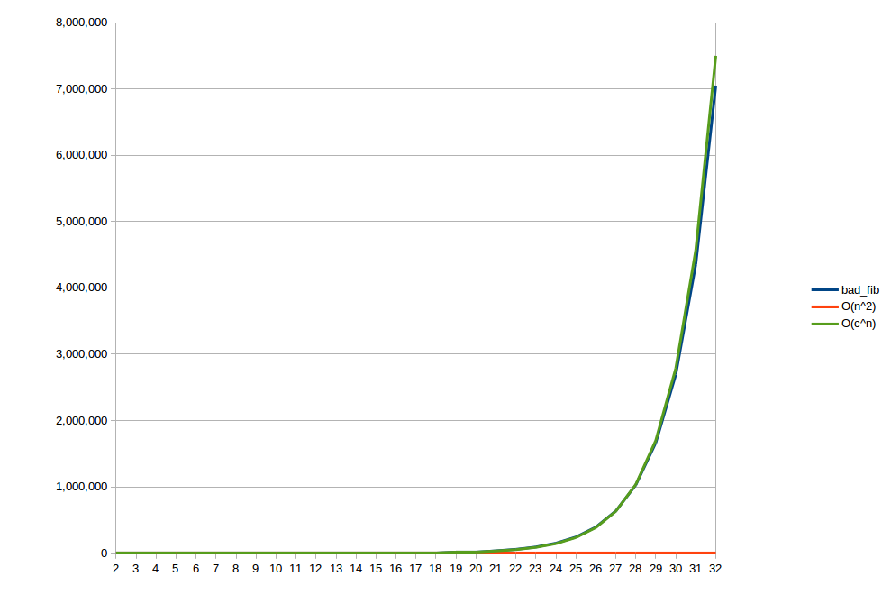
First approach seems to be somewhere around O(1.65n)
Second approach is O(n)
To make matters worse, the first approach also takes a significant amount of
memory on the stack. If you use memoization to reduce the run-time, you still take
O(n) memory. The second approach is linear in time with a constant
memory footprint. Memoizing the second approach turns it from linear in time to
linear in space.
Summary
- If input size is small, algorithm normally doesn't matter much.
- If the code is only run once, algorithm usually doesn't matter.
- Profile if possible to gain understanding and find bottlenecks.
- Change in algorithm can still be readable, unlike micro-optimizations.
In a particular piece of code, if you have a linear piece, followed by a quadratic piece, the quadratic piece dominates for large inputs. The higher order piece always dominates. Nested levels multiply.
Summary, 2
- Use analysis if profiling is impractical.
- Use analysis for easy wins.
- Use analysis to check your assumptions.
- Don't try to analyze really complicated algorithms.
- ... but divide and conquer may help here as well.
Use analysis to reduce your work. Check intuition about code with simple analysis. Use the analysis to explain results of profiling. If the algorithm is really complicated, measure rather than analyze.
Wikipedia References
- Time complexity - Wikipedia, the free encyclopedia
- Analysis of algorithms - Wikipedia, the free encyclopedia
- Big O notation - Wikipedia, the free encyclopedia
- Best, worst and average case - Wikipedia, the free encyclopedia
Other References
- Complexity
- Complexity of an Algorithm
- Big-O Algorithm Complexity Cheat Sheet
- A Gentle Introduction to Algorithm Complexity Analysis
- 1.2 Complexity of Algorithms
Questions?
Details of Fibonnaci Example

| n | bad | good | O(n2) | O(1.64n) |
|---|---|---|---|---|
| 2 | 3 | 2 | 4 | 3 |
| 3 | 5 | 3 | 9 | 4 |
| 4 | 9 | 3 | 16 | 7 |
| ... | ... | ... | ... | ... |
| 10 | 177 | 10 | 100 | 141 |
| 11 | 287 | 11 | 121 | 231 |
| ... | ... | ... | ... | ... |
| 20 | 21,891 | 20 | 400 | 19,810 |
| ... | ... | ... | ... | ... |
| 31 | 4,356,617 | 31 | 961 | 4,572,559 |
| 32 | 7,049,155 | 32 | 1,024 | 7,498,996 |
This shows some of the measurements I used to work out the order of the fibonacci algorithm. I mostly played around with numbers and eyeballed the curve fit.